Chapter 11. Chemical Plume and Dispersion Analysis
11.1. Chemical Plume Dispersion Analysis
11.2. Chemical Plume Dispersion Analysis(contd.)
11.3. Identifying the Source
11.4. Release
11.5. Possible Release Mechanisms
11.6. Source Characterization
11.7. Source Characterization(contd.)
11.8. Catastrophic Rupture
11.9. Continuous Liquid Release
11.10. Bernoulli Equation
11.11. Continuous Gas Release
11.12. Flashing Liquids
11.13. Instantaneous Vapor Release
11.14. Liquid Pool Evaporation and Vaporization
11.15. Liquid Pool Surface Area Calculation
11.16. Evaporation Rate Calculation
11.17. Evaporation Rate Calculation(contd.)
11.18. Dispersion Modeling
11.19. Heavy Gas Dispersion
11.20. Heavy Gas Dispersion
11.21. Transport Processes in a Plume
11.22. Neutrally Buoyant Gases
11.23. Estimating Chemical Concentrations with a Gaussian Plume Model
11.24. Model Performance and Uncertainty
11.25. Gaussian Plume Model Assumptions
11.26. Gaussian Plume Model Assumptions and Accuracy
11.27. Hazardous Material Models
11.28. Air Emissions
11.29. Air Emissions(contd.)
11.30. Air Emissions(contd.)
11.31. Estimating Air Emissions
11.32. Estimating Air Emissions(contd.)
11.33. Estimating Air Emissions(contd.)
11.34. Estimating Air Emissions(contd.)
11.35. Estimating Air Emissions(contd.)
11.36. Estimating Air Emissions(contd.)
11.37. Estimating Air Emissions(contd.)
11.1. Chemical Plume Dispersion Analysis
Dispersion modeling of potential releases of hazardous chemicals is an integral part of risk management. It forms the link between the potential equipment failure and the consequences that would be suffered by plant personnel and the public. There are numerous models of varying sophistication to predict the transport of a hazardous chemical. The material presented here will provide a description of the methods for analyzing hazardous chemical dispersion for risk assessment and describe problems and constraints in conducting these evaluations. This will provide insight and assistance in the use of available methods and models.
11.2. Chemical Plume Dispersion Analysis (continued)
Chemical plume dispersion analysis models postulate accidental releases of hazardous chemicals. This includes estimating hazardous vapor concentrations within and beyond plant boundaries to help quantify risks. It forms the critical link between the hypothesized equipment failures or release scenarios and the potential consequences suffered by plant personnel and the public.
11.3. Identifying the Source
The first step in dispersion analysis is identifying the source
The first step in dispersion analysis is to identify the source. Also, the source or sources of a potential vapor release must be characterized. This leads to identifying some important terms associated with chemical plume dispersion analysis as given on the next slide.
11.4. Release
May originate from any number of plant components including storage tanks, reactors, and piping
A release may originate from any number of plant components including storage tanks, reactors, and piping. Some release mechanisms are shown on the next slide.
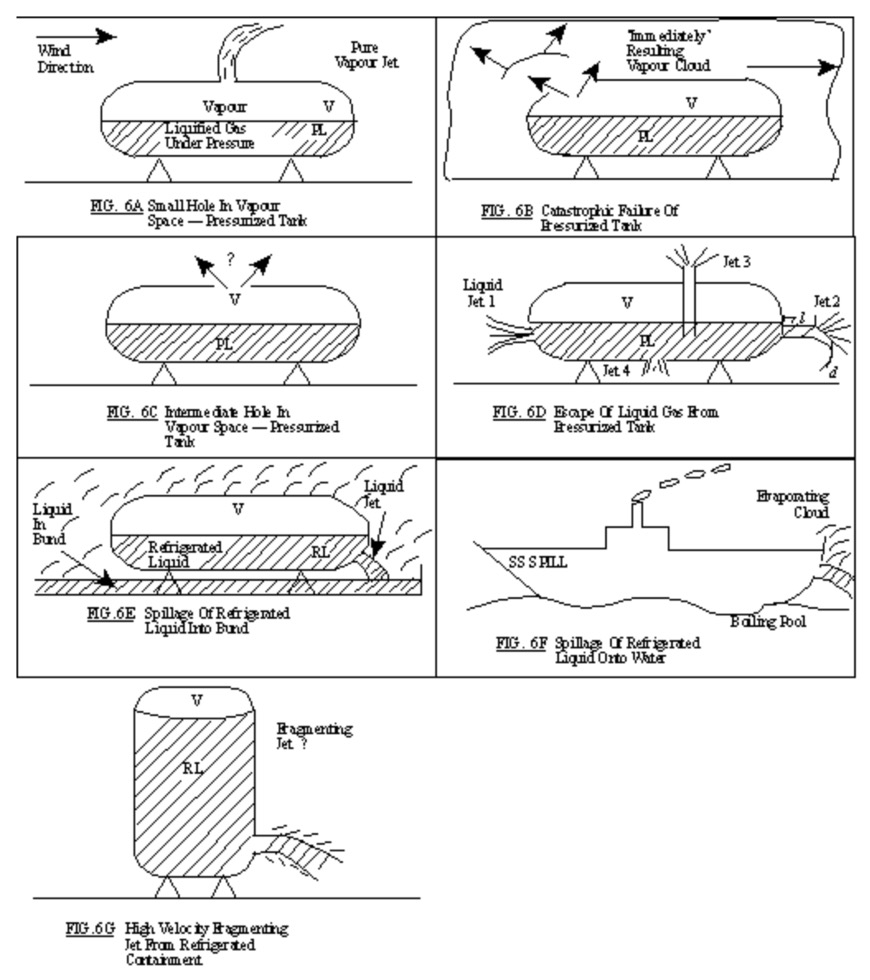
11.5. Possible Release Mechanisms
Here are a few examples of possible release mechanisms. In the first picture, you see a small hole in the vapor space-pressurized tank. In Figure B, the tank fails. In the next scenario, Figure C, there is an intermediate hole in the vapor space-pressurized tank. In Figure D, we see that liquefied gas from the tank escapes. In the next scenario, we see that refrigerated liquid is spilled, and this result can be seen in Figure F, where the refrigerated liquid spills into the water. Figure G shows another scenario where there is a high velocity fragmented jet from the refrigerated container.
11.6. Source Characterization
To determine a source strength as a function of time, examine:
Source characterization refers to determining the source strength with time. The information of this evaluation is listed on the slide and includes physical and chemical characteristics of the stored material, the geometry of the source and plant operating procedures.
11.7. Source Characterization (continued)
Also examine:
Source characterization also includes the evaluation shown. These include spill surface characteristics, meteorological data and site characteristics.
11.8. Catastrophic Rupture
Must use the assumption of an instantaneous release for dispersion modeling
A catastrophic rupture scenario would equate to a tank rupturing. In this scenario, you assume instantaneous release of the contents.
An example of a continuous release would be the case where a hole is punched in the liquid portion of a pressurized or refrigerated storage vessel as shown in this diagram.
11.9. Continuous Liquid Release
To determine liquid release rate from a storage vessel, use Bernoulli’s Equation. Bernoulli’s equation is used to predict the flow rate from the tank as shown on the next slide.
Another scenario has the liquid spill on the ground spreading into a large pool. A ground level vapor plume is generated. The discharge rate from the tank is dependent on the pressure in the tank, the liquid level and the size of the hole.
11.10. Bernoulli Equation
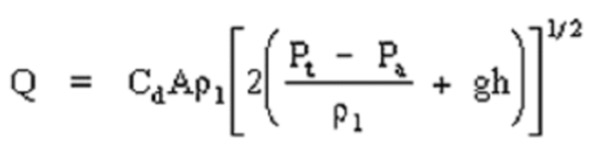
where:
Q = liquid release rate (Kg/sec)
Cd = discharge coefficient (dimensionless)
P1 = density of the liquid (Kg/m3)
A = area of puncture (m2)
Pt = tank pressure (n/m2)
Pa = atmospheric pressure (n/m2)
g = gravitational acceleration (9.8 m/sec2)
h = liquid head (m)
In this continuous liquid release scenario, the discharge rate can be determined from the Bernoulli equation. Here a typical value for Cd for puncture or pipe break would be 0.8.
11.11. Continuous Gas Release
Characterized as critical or sub critical
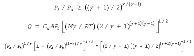
For a continuous gas release, the release usually occurs in the form of a jet that is characterized as critical or sub-critical flow. Critical or 'choked' flow is the maximum flow rate regardless of the up stream pressure, and the velocity can not exceed the velocity of sound. For these conditions, the volumetric flow rate Q is given by the equation shown here. When the flow becomes sub-critical, the equation for Q is multiplied by the factor shown on the third line of this slide.
11.12. Flashing Liquids
Mv/Mo = (Cp/Hv) (Ts-Tb)
where
Mv= mass of vapor due to flashing (Kg)
Mo= total liquid mass (Kg)
Cp= specific heat at constant pressure (J/Kg/oK)
Hv= Heat of vaporization (J/Kg)
Ts= storage temperature (oK)
Tb= liquid boiling point (oK)
Flashing Liquids have low boiling points and may instantaneously flash a portion of the liquid into vapor. The vapor fraction can be determined with this heat balance equation by assuming the vaporization portion to be adiabatic. The vapor cloud is taken to be at the boiling point with gradual warming as ambient air is entrained into the cloud.
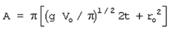
11.13. Instantaneous Vapor Release
![]()
Assume instantaneous release and a spherical puff
For instantaneous vapor release from a flashing liquid described on the previous slide, the radius of the cloud can be estimated from this equation. It assumes that the cloud is spherical.
11.14. Liquid Pool Evaporation and Vaporization
Another important source of chemical emissions is the liquid pool formed by the spill of chemical with a boiling point above ambient temperature. Also, it can be that heavier part of a low boiling point liquid mixture that does not flash off. In either case, the first step in estimating emission rates is to estimate the size of the puddle as it spreads on the ground, as shown on the next slide. Then you can estimate the rates due to evaporation or vaporization.
11.15. Liquid Pool Surface Area Calculation
Basis: a cylinder with height equal to the radius of the base
First, the surface area of the liquid pool is detrmined the using the above equation. The liquid pool surface area calculation is based on a cylinder with height equal to the radius of the base.
11.16. Evaporation Rate Calculation
For a liquid with a boiling point above ambient temperature
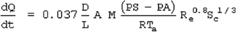
where
dQ/dt = vapor emission rate (Kg.sec)
D = diffusion coefficient (m2/sec)
L = characteristic length (m)
If the spill is a liquid with a boiling point above the ambient temperature, the rate of evaporation can be estimated by this equation which is based in forced convection. A value for the diffusion coefficient of 0.002 m2/ sec is recommended if one is not available from the literature.
11.17. Evaporation Rate Calculation
For a liquid with a boiling point below ambient temperature
![]()
Evaporation rate is the sum of the heat transferred to the liquid by conduction, radiation and convection divided by the heat of vaporization. Conduction usually dominates.
where
qd = heat transfer rate (watts)
Ks = thermal conductivity of the soil (watt/m/oK)
Tc = soil temperature (oK)
Tb = chemical boiling point (oK)
pe = density of earth's crust (Kg/m3)
Cpe = heat capacity of the earth's crust (J/Kg/oK)
For a liquid with a boiling point below ambient temperature the evaporation rate is the sum of the heat transferred to the liquid by conduction, radiation and convection divided by the heat of vaporization, dQ/dt = (qd + qr + qc)/Hv. Conduction usually dominates and the equation given on the slide is the one to use to estimate this value, qd. A conservative value for radiation, qr, is 1,200 watts/m2. For convection, the rate, qc, is estimated by a heat transfer coefficient times the difference in the ambient and liquid pool temperatures. A conservative value for the heat transfer coefficient is 7.0 watts/m2/K.
11.18. Dispersion Modeling
Instantaneous and continuous releases require different methods
Now that we have examined source of the release, we can begin to address the actual dispersion of the release. We will discuss the common approaches used in simulating dispersion mechanisms. There are different ways of describing and evaluating instantaneous and continuous releases. Jet releases are those from tank and pipeline ruptures, and the plume depends on the vapor's physical properties. The jet from this type of release can be described by a Gaussian plume. Heavy gas releases require a more detailed model than the Gaussian plume model. Neutrally buoyant gases are dispersed by atmospheric turbulence, and a Gaussian plume mode
1.19. Heavy Gas Dispersion
We will begin with the heavy gas dispersion which is density driven. The weight of the cloud causes it to slump and spread out in all directions. The rate of spread of the cloud can be estimated by an equation given on the next slide.
11.20. Heavy Gas Dispersion
Equation for Estimating Rate of Cloud Spread
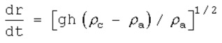
This equation is based on the cloud forming a cylinder of height h.
This is the equation used for heavy gas dispersion. It gives the rate that the cloud spreads, and it is based on the cloud forming a cylinder of height h.
11.21. Transport Processes in a Plume![]()
Transport processes in a plume are show in this diagram. Moment transport includes mixing of the plume with ambient air. Heat Transfer includes conduction to the ground, convection with mixing, and radiation from the sky, for example. Mass transport includes diffusion, dispersion, and evaporation of plume species. Chemical reaction kinetics determines the rate of formation of new species from the plume species and air species.
11.22. Neutrally Buoyant Gases
There is a point during dispersion where density-driven turbulence becomes weak, and atmospheric turbulence becomes more significant. After this transition point, the dispersion distance may be approximated by using a point source with a Gaussian plume model. The application of a Gaussian plume model will be illustrated on the next slide.
11.23. Estimating Chemical Concentrations with a Gaussian Plume Model
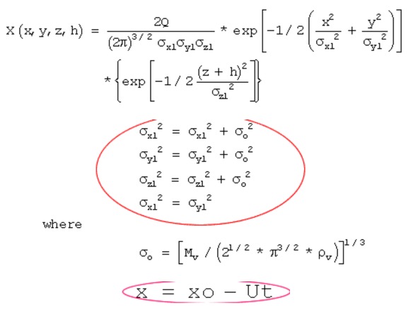
For a puff release with an initial finite volume, the chemical concentration X(x,y,z,h) in the puff is described by this equation. Note that the initial volume of the puff is accounted for by adjusting the standard deviations of concentration as shown in the red circle. Also, the value of x in the exponential term is determined by x = xo – Ut, which is the distance between the source of the spill and the receptor. U is the wind speed. An application of this model is given in the Health Effects section to predict the concentration distribution of a hazardous chemical.
11.24. Model Performance and Uncertainty
Gaussian Model:
Dispersion models are approximate because they cannot completely account for the randomness and uncertainties associated with the actual dispersion process. To make the calculations in the model manageable, the physical equations are solved by assuming steady-state conditions and using empirically derived parameters to close the set of equations. The Gaussian model provides a simplified solution for the dispersion problem. However, in order to use the Gaussian model, several assumptions must first be met as shown on the next slide.
11.25. Gaussian Plume Model Assumptions
This slide lists some of the assumptions that were used to obtain a solution for a Gaussian plume. Others are shown on the next slide.
11.26. Gaussian Plume Model Assumptions and Accuracy
There have been numerous studies to evaluate the precision of the Gaussian plume model to describe actual plumes from releases. Results have shown that if the terrain, meteorological conditions, release rate and other conditions were close to the assumptions for the model, the accuracy was within a factor of two when comparing predicted concentrations with field measurements. If the restrictions were not met approximately, the comparison was within a factor of ten.
11.27. Hazardous Material Models
Constraints:
In the case of hazardous material models, there are additional constraints that add to further uncertainty in predictions. These constraints are listed here, and they are heavy gas dispersion, non-steady-state releases, and aerosol formation.
11.28. Air Emissions
Four general categories of emission sources:
Air emissions from chemical plants come from dilute concentrations in large vent streams; from vapor emissions from “breathing” storage tanks; from fugitive emissions from process equipment, for example valves, shafts and flanges; and accidental releases.
11.29. Air Emissions (contd.)
When new liquid is added, vapor is displaced to the atmosphere
Examples of emissions from large vent streams and vapor emissions are shown here. These are difficult to eliminate.
11.30. Air Emissions (contd.)
To illustrate the magnitude of these emissions from a chemical plant, estimate the amount of acetic acid vapor that would be vented to the atmosphere during the filling of a 10,000 gallon fixed-roof tank. Assume there are no vapor recovery controls on the tank and that the operation takes place at an ambient temperature of 70 deg F. The vapor pressure of acetic acid at 70 deg F is 12.24 mm Hg. Its molecular weight is 60.05.
Compare your results with the evaluation given on the next slide.
11.31. Estimating Air Emissions (contd.)
Calculate the mass of acetic acid vapor in equilibrium with liquid which will occupy a volume of 10,000 gallons.
Assume the vapor space in the tank rapidly reaches equilibrium with the first few gallons of acetic acid liquid.
Convert the volume of the tank to ft3.
There are 7.481 gallons per cubic foot.
V = 10,000 gal = 1337 ft3
Convert the vapor pressure to psia and the temperature to oR.
There are 51.7 mm Hg per psi. Adding 460 converts oF to oR.
Pv = 12.24 mm Hg = 0.237 psia, T = 73 oF = 530 oR
Use the ideal gas law to calculate the total amount of acetic acid vapor in the tank.
Apply the ideal gas law to calculate the moles of acetic acid.
N = PvV/RT = (0.237) (1337) /(10.73)(530). = 0.0556 lb moles
Convert the moles to mass
N = (0.0556) (60.05) = 3.34 lb
Assume the vapor space is filled with acetic acid vapors left from emptying the tank. Then use the ideal gas law to determine the number of moles of acetic acid in the tank and convert the moles to mass.
11.32. Estimating Air Emissions (contd.)
This slide describes standard procedures for filling and emptying atmospheric tanks. Federal and state regulations set the limits on emissions to the atmosphere from these operations and when end-of-pipe treatment is required.
11.33. Estimating Air Emissions(contd.)
A nitrogen blanket is frequently used to prevent an explosive mixture from forming on tanks filled with hydrocarbons and also to reduce emissions. Evaluate emissions from the filling of a tank with cyclohexane as shown on this slide. Additional information is given on the next slide.
11.34. Estimating Air Emissions(contd.)
Evaluate the amount of cyclohexane vapor emitted to the atmosphere if:
This evaluation is typical of ones that have to be performed for tanks. The results are used in an economic analysis to determine a return on investment for a compressor and to comply with environmental regulations.
11.35. Estimating Air Emissions(contd.) Data
- Molecular Weight - 84.16
- Vapor pressure @ 80oF - 2.051 psia
- Vapor pressure @ 85oF - 2.320 psia
Use this information to calculate the pounds of cyclohexane released with and without treatment. Compare your results with the evaluation given on the next slide
11.36. Estimating Air Emissions(contd.)
Calculate the total number of moles of gas in 2,000 bbl at 80oF and 1.00 atm.
Use the ideal gas law. Remember that one barrel (bbl) is 5.614 ft3.The mole fraction of cyclohexane will be the same as the ratio of its vapor pressure to the total pressure.
For Case 1, calculate the lb moles of cyclohexane and of inert gas in the released gas.
For Case 2, calculate the moles of cyclohexane that will still be vapor at 85oF and 100 psia.
Again, the mole fraction of cyclohexane will be the same as the ratio of its vapor pressure to the total pressure. The number of moles of inert gas will be the same as in Case 1.
For each case, convert the results to lbs of cyclohexane.
Multiply the masses by the molecular weights.
With no treatment 334 pounds of cyclohexane are released every time the storage tank is filled. With the vapor recovery system, only 50 pounds are released. See the next slide for calculations.
11.37. Estimating Air Emissions(contd.)
Calculate the total number of moles of gas in 2,000 bbl at 80oF and 1.00 atm
NT = PV/RT = (14.7) (2000 x 5.614)/(10.73 x 540) = 28.48 lb moles
For Case 1, calculate the lb moles of cyclohexane and of inert gas in the released gas.
Nc1 = (NT)(Pc/PT) = (28.48) (2.051/14.7) = 3.97 lb moles
Pi = PT - Pc = 14.7 - 2.051 = 12.649 psia
Ni = (NT)(Pi/PT) = (28.48) (12.649/14.7) = 24.51 lb moles
For Case 2, calculate the moles of cyclohexane that will still be vapor at 85oF and 100 psia.
Pi = PT - Pc = 100.0 - 2.320 = 97.68 psia
Nc 2 = (NT)(Pc/PT) = (28.48) (2.051/14.7) = 3.97 lb moles
For each case, convert the results to lbs of cyclohexane.
Mc1 = (3.97) (84.16) = 334 lb
Mc2 = (0.582) (84.16) = 50 lb
This slide gives the procedure used and the numerical values for the two case.